There are two major classes of probability distributions: Discrete and Continuous. A discrete random variable has a finite or countable number of possible values, for exemple the number of codons that code a certain amino acid, how many CG diagrams are observed in a DNA sequence, the different blood types or genotypes in a population etc…
Bernoulli trials and Binomial Distributions
Bernoulli Trials
A Bernoulli trial is defined as an experiment with only two possible outcomes labeled success (p=1) and failure(p=0).
You can think of the two possible outcomes as : mutation or no mutation, CpG or no CpG, intron or exon, purine or pyrimidine, female or male…
Some other discrete probability distributions are built on the assumption of independent Bernoulli trials.
Binomial distributions
Okay, brace yourselves, there are some mathematical formula that are coming but don’t run yet, they are more simple than you might think and they will grant you some superpowers like predicting mutation !
X∼B(n,p)
The above formula can be translated in plain english as: the variable X follows a Bionomial distribution with n (Bernoulli) trials and a probability of success equal to p.
A binomial distribution is a distribution that arises from a number of successes in n independent Bernoulli trials. The distribution hence has two parameters: the number of trials (n) and success probability in each trial (p).
Notes for the terrified:
- A distribution is the shape that you your data takes when you plot it. (very informal definition.)
- Binomial means that there are two possible outcomes as opposed to multinomial distributions where there are more than two outcomes (in the case of DNA for exemple, at any given position you have for possible bases, blood types and genotypes are also great exemples).
- By Independant trials we mean that knowing the result of one trial gives you no information about the outcome of another trial.
- The probability of success p, is always a number between 0 and 1 (inclusive).
Exemple : Drug success.
Suppose you want to study the effect of a drug and want to know if treating patients with it will have any effect.
The outcomes are either: success (patients will report relief) or failure
(patients will report no relief). Hence, reporting the result of a patient is a Bernoulli trial.
Reporting the results of a group of patients is on the other hand is a series of Bernoulli trials and will give rise to a Binomial disribution.
Time for some plots and some r programming to see the theroy in action.
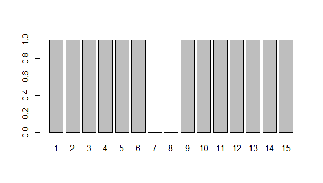
Say that 75% of patients treated with your medecine reported relief. Let us simulate a sequence of 15 patients treated with that medication:
## Setting the seed to ensure the your code and mine will look identical
set.seed(10000)
rbinom(n=15, prob = 0.75, size = 1)
## [1] 1 1 1 1 1 1 0 0 1 1 1 1 1 1 1
rbinom() is the r function that lets you do so. It takes three parameters:
- n: the number of observations.
- prob: the probability of success.
- size: the sample size.
You can check how many successes you’ve reported and how many failures using the table function:
set.seed(10000)
table(rbinom(15, prob = 0.75, size = 1))
##
##  0  1
##  2 13
R lets you also plot your data:
set.seed(10000)
barplot(rbinom(15, prob = 0.75, size = 1), names.arg = 1:15)
To compute the probability of seeing (X=k) successes you need to apply the following formula:
P(X=k) =
For the drug exemple, suppose you want to know the probability of getting 10 successes in n= 15 trials.
choose(15,10) * (0.75 **10 ) * (1-0.75) ** 5
0.165146
Notes for the terrified:
- If you are not familiar with counting, you may find this formula strange:
. You read it n choose k, the choose() function in r computes the value for you as you've seen it in the code snippet above. I will probably write an article about counting soon since it is a really important -and fun- topic.
Poisson distributions
Another useful discrete distribution is the well-known Poisson distribution. Remember when we defined the binomial distribution as being a distribution that arises from a sequence of n independant Bernoulli trials ?
Well the Poisson distribution is exactly the same, the only difference is that it is used when the probability of success p is very small (ie. ) and the number of trials n is large(ie.
).
It has only one paramterer: , such as
=np.
Thus, the Poisson distribution is used to describe rare events in a large population such as mutation aquisition in a large set of cells.
Exemple: Mutation in the human genome
The human genome mutation rate is approximately p=1.1×10⁻⁸ per site per generation.[1]. The diploid genome size is n=6.3 x 10 9. This model predicts that the number of mutations over one generation will be = (1.1×10⁻⁸ )x 6.3 x 10 9 = 69.3.
If you want to know the probability of having 39 mutations under a Poisson distribution with = 69.3 can be computed with the following formula: P(X=k) =
dpois(x = 39, lambda = 69.3)
2.412145e-05
Conclusion:
And that’s it for today! Stay connected if you want to learn more of biostatistics for the terrified.